


Abstract
Metabolomics is a potentially powerful tool for identification of biomarkers associated with lifestyle exposures and risk of various diseases. This is the rationale of the ‘meeting-in-the-middle’ concept, for which an analytical framework was developed in this study. In a nested case–control study on hepatocellular carcinoma (HCC) within the European Prospective Investigation into Cancer and nutrition (EPIC), serum 1H nuclear magnetic resonance (NMR) spectra (800 MHz) were acquired for 114 cases and 222 matched controls. Through partial least square (PLS) analysis, 21 lifestyle variables (the ‘predictors’, including information on diet, anthropometry and clinical characteristics) were linked to a set of 285 metabolic variables (the ‘responses’). The three resulting scores were related to HCC risk by means of conditional logistic regressions. The first PLS factor was not associated with HCC risk. The second PLS metabolomic factor was positively associated with tyrosine and glucose, and was related to a significantly increased HCC risk with OR = 1.11 (95% CI: 1.02, 1.22, P = 0.02) for a 1SD change in the responses score, and a similar association was found for the corresponding lifestyle component of the factor. The third PLS lifestyle factor was associated with lifetime alcohol consumption, hepatitis and smoking, and had negative loadings on vegetables intake. Its metabolomic counterpart displayed positive loadings on ethanol, glutamate and phenylalanine. These factors were positively and statistically significantly associated with HCC risk, with 1.37 (1.05, 1.79, P = 0.02) and 1.22 (1.04, 1.44, P = 0.01), respectively. Evidence of mediation was found in both the second and third PLS factors, where the metabolomic signals mediated the relation between the lifestyle component and HCC outcome. This study devised a way to bridge lifestyle variables to HCC risk through NMR metabolomics data. This implementation of the ‘meeting-in-the-middle’ approach finds natural applications in settings characterised by high-dimensional data, increasingly frequent in the omics generation.
Introduction
Metabolomic profiles from blood and other biological samples collected from large-scale epidemiologic studies are increasingly being investigated (1), following recent developments in nuclear magnetic resonance (NMR) and mass spectrometry (MS) enabling the assessment of metabolic profiles for large numbers of individuals. As a result, metabolomic data is gradually playing a key part in clinical and observational studies; and new statistical methodologies (2) are increasingly being sought to explore insights into pathological processes that metabolomics may provide in order to better understand determinants of disease development. These approaches explore a variety of aetiological hypotheses; however, they usually focus on one aspect at a time, combining metabolomics with either epidemiologic/phenotypic data on lifestyle exposures (3) or with disease outcomes (4,5). The main aim of this work is to jointly use all aspects that are potentially informative to apprehend the contrivances of disease development.
Metabolomic data offers the opportunity to identify signatures and biomarkers associated with environmental exposures and the risk of a disease. Prospective studies are conceptually suitable for this purpose, since they rely on biological samples collected before disease onset, and are thus marginally influenced by metabolic changes due to processes of disease development. In this scenario, the ‘meeting-in-the-middle’ (MITM) approach (6) has been conceived as a research strategy to identify biomarkers that are related to specific exposures and that are, at the same time, predictive of disease outcome. Finding this overlap between exposure and disease of ‘intermediate’ biomarkers can potentially disclose useful information on the exposure-to-disease pathway, and may serve as an objective risk exposure measure, ultimately allowing the identification of a targeted prevention scheme. The MITM was previously implemented as a proof of concept in a case–control study nested within a cohort of healthy individuals (7), where a list of putative intermediate 1H NMR biomarkers linking exposure to dietary compounds, mainly micro- and macronutrients, and disease outcomes (colon and breast cancer) were investigated.
In this study, we extend previous attempts to model the MITM by fully integrating metabolomics, lifestyle and disease risk in a single analytical framework. A strategy was developed to simultaneously investigate a broad range of metabolites and lifestyle variables with a partial least square (PLS) regression model (8). The resulting scores were related to the risk of hepatocellular carcinoma (HCC), in a case–control study nested within the European Prospective Investigation into Cancer and nutrition (EPIC). HCC is the most frequent primary form of cancer affecting the liver, an organ that plays a critical role in many metabolic pathways (9). HCC is a disease with multifactorial origins embracing lifestyle and dietary exposures whose intersection may reveal metabolomic signals (10) relevant to cancer onset. The system of relationships between metabolomic profiles and lifestyle factors in relation to HCC was evaluated by means of mediation analysis. The methodological challenges characterising the analysis of large and complex metabolomic datasets are described and discussed.
Methods
EPIC design
The European Prospective Investigation into Cancer and nutrition (EPIC) is a large cohort established to investigate the association of diet, lifestyle and environmental factors with cancer incidence and other chronic disease outcomes. Between 1992 and2000, over 520 000 participants aged 20–85 years, were recruited from 23 centres in 10 Western European countries including Denmark, France, Germany, Greece, Italy, Norway, Spain, Sweden, the Netherlands and UK (11). The design, rationale and methods of the EPIC study including information on dietary assessment methodology, blood collection protocols and follow-up procedures were discussed previously (11).
Between 1992 and 1998, standardised lifestyle data, anthropometric measures and biological samples were collected at recruitment, prior to onset of any disease (11). Validated country-specific questionnaires ensuring high compliance were used to measure diet over the previous 12 months (12). Blood samples are stored at the International Agency for Research on Cancer (IARC, Lyon, France) in −196ºC liquid nitrogen for all countries, exceptions being Denmark (nitrogen vapour, −150ºC) and Sweden (freezers, −80ºC).
The nested case–control study
The present study focused on data with available sera samples from a nested case–control study in EPIC on HCC (13). Cases of HCC were identified from all participating EPIC centres except for Norway and France (n = 117) from recruitment (1993–1998) up to 2007. Two controls (n = 232) were selected for each case from all cohort members alive and free of cancer (except non-melanoma skin cancer) by incidence-density sampling and were matched on age at blood collection (±1 year), sex, study centre, date (±2 months), time of the day at blood collection (±3h) and fasting status at blood collection (<3, 3–6, >6h); among women, additional matching criteria included menopausal status (pre-, peri-, post-menopausal) and hormone replacement therapy (HRT) use at time of blood collection (yes/no). In the present study, cases and controls were both included in the analyses as the subjects were all cancer-free at blood collection. Out of the total 349 subjects, 7 subjects (3 cases and 4 controls) had too little serum volume for NMR spectral acquisition with sufficient sensitivity; 6 additional control subjects were excluded following the exclusion of their corresponding case subject. The final analysis included 114 HCC cases and 222 matched controls of which 108 case–control sets with two matched control subjects and 6 sets with one matched control subject.
NMR spectra acquisition
Sera were processed using standard procedure for 1H NMR metabolic measurement and profiling protocols (14). Details on the sera sample preparation as well as NMR data acquisition and processing have been described elsewhere (15). In brief, each spectrum was reduced to 8500 bins of 0.001 ppm width over the chemical shift range of 0.5–9 ppm. Spectra were normalised to total intensity, centred and Pareto scaled, and additionally normalised for batch effects using the batch profiling calibration method (16). After removal of the structured noise (characterised by a specific mean and standard deviation) located in a well-known noise region (8.5–9 ppm) and variables with identical characteristics, the statistical recoupling of variables (SRV) (17), a bucketing procedure, was applied to the metabolomic spectra. The SRV procedure identifies clusters of variables with respect to the ratio of covariance and correlation between consecutive variables along the chemical shift axis, allowing the restauration of the spectral dependency and the recovery of complex NMR signals corresponding to potential physical, chemical or biological entities. More details on the SRV procedure are available in the Supplementary Appendix, available at Mutagenesis Online. This permitted a reduction of the number of NMR variables from 8500 bins to 285 clusters of variables corresponding to reconstructed peak entities which constituted the Y-set of metabolic variables. All steps to obtain the data were done without knowledge of the case–control status of the subjects. Quality control (QC) samples were included to ensure reproducibility of the NMR data acquisition.
Metabolite identification
The assignment of NMR signals observed in the 1H one-dimensional fingerprints to metabolites has been achieved by the analysis of additional 2D NMR experiments 1H–13C HSQC and 1H–1H TOCSY obtained on a subset of representative samples (one control and one case). The measured chemical shifts were compared to reference shifts of pure compounds using HMDB (18), MMCD (19) and ChenomX (ChenomX NMR suite, ChenomxInc, Edmonton, Canada) databases.
Lifestyle variables
The predictors (what will be referred to later on as the X-set) included 13 dietary variables from main EPIC food groups compiled from validated country-specific food frequency questionnaires (FFQ) (11,20) (potatoes and other tubers; vegetables; legumes; fruits, nuts and seeds; dairy products; cereal and cereal products; meat and meat products; fish and shellfish; egg and egg products; fat; sugar and confectionary; cakes and biscuits; non-alcoholic beverages), alcohol average lifetime intake (continuous, g/day), anthropometric measures including body mass index (continuous, kg/m2) and height (continuous, cm) that were measured by trained interviewers in the majority of participants (11), highest level of education achieved (categorical: none or primary school completed, technical/professional school, secondary school, longer education (incl. university degree), unspecified), smoking status (categorical: never, former, current smoker, unknown), a measure of physical activity (continuous, metabolic equivalents of task (MET)/h), hepatitis status [yes/no, from biomarker measures of HBV and HCV seropositivity (ARCHITECT HBsAg and anti-HCV chemiluminescent microparticle immunoassays; Abbott Diagnostics, France)] and baseline self-reported diabetes status (yes/no). Descriptive information on these variables can be found in Supplementary Table 1, available at Mutagenesis Online.
Statistical analyses
PC-PR2 analysis
Principal component partial R-square (PC-PR2) was primarily used to identify and quantify sources of systematic variability within metabolomic data (15). PC-PR2 combines aspects of principal component analysis (PCA) and the R2partial statistic in multiple linear regression, and allows for (some) intercorrelation between the explanatory variables under scrutiny (15). In short, PCA is performed on the 285 clusters of 1H NMR variables and a number of components is retained explaining an amount of total variability above a designated threshold (here, 80%). Then, multiple linear regression models are fitted where each component’s variability is explained in terms of relevant covariates, e.g. specific characteristics of samples like country of origin, smoking status, laboratory treatment, etc. For each given component, the R2partial statistic is computed for all covariates, quantifying the amount of variability each independent variable explains, conditional on all other covariates included in the model. Finally, an overall R2partial is calculated as a weighted average for every covariate, using the eigenvalues as components’ weights. Mathematical details pertaining to the PC-PR2 method are described elsewhere (15).
In this study, PC-PR2 was applied to the 285 clusters of NMR variables, whereas the explanatory variables examined for systematic variability were NMR batch, country of origin, sex, age at blood collection, serum clot contact time (centrifugation at the day of blood collection d, or the following day, d + 1), length of freezing time (≤15 vs. >15 years), and fasting status at blood collection (< 3, 3–6, > 6h). With the similar motivation of identifying sources of variability within lifestyle data, a similar PC-PR2 analysis was applied to the 21 lifestyle factors, the examined covariates for systematic variability were country of origin, sex and age at recruitment. For both metabolomics and lifestyle data, residuals on the variable accounting for most variability, identified through PC-PR2 analyses, were computed in a series of univariate linear regression models (21) and were used in the subsequent PLS.
PLS analysis
A PLS model was used to relate lifestyle variables to metabolomic profiles. PLS is a multivariate technique that generalises features of PCA and multiple linear regression. PLS iteratively extracts linear combinations of, in turn, predictors (the X-set) and responses (the Y-set), which in this study, were lifestyle variables and metabolomic profiles, respectively. First, components or latent factors are extracted allowing a simultaneous decomposition of the X- and Y-sets, in order to maximise their covariance (22). The factors extracted from the predictors’ set are orthogonal. Computational details of PLS are described in the Supplementary Appendix, available at Mutagenesis Online. As a standard step for the PLS algorithm, the X- and Y-sets were centred and standardised for the analysis and a simple expectation–maximisation (EM) algorithm, adapted from the PLS kernel algorithm (23,24), was used to compute covariance matrices when missing values were present in the lifestyle data. This was done as follows: a first pass of PLS was computed filling in the missing values by the average of the non-missing values for each corresponding variable. A second pass was then performed whereby the missing data were assigned their predicted values based on the first model, and the PLS regression is recomputed.
Then, a 7-fold cross validation analysis was carried out to select the number h of significant PLS factors to retain (8) (see Supplementary Appendix, available at Mutagenesis Online). This was achieved by splitting the data into seven groups of observations. In turn, each group of observations was considered as the test set, while the other six were the training sets, used to perform PLS analysis. A measure of PLS performance was determined for each step through the predicted residual sum of squares (PRESS) statistic, whereby the predicted values in the test set, the Ỹh matrix, based on the X-components estimated through the model in the training set, were compared to the observed responses, the Y matrix. This comparison is quantified by the squared Euclidean distance between these two matrices. In turn for an increasing number h of components, the process is iterated seven times, until each group of observations serves as a test set. Eventually, the number h of selected PLS factors is the one minimising the PRESS statistic.
For each PLS factor, loadings were computed for the lifestyle (X-set) and the NMR (Y-set) variables. The loadings, i.e. coefficients quantifying the contribution of each original variable to the PLS factor, were used to characterise the various factors. As the analysis involved many variables in the X-set and, particularly, in the Y-set, the interpretation focused primarily on variables with loading values lower than the 10th percentile and larger than the 90th percentile for the X variables, and lower than the 5th and larger than the 95th percentiles for the Y variables, that were deemed the most significant contributors to the PLS factor.
Logistic regression analysis
Last, scores of each PLS factor were related to HCC risk in conditional logistic regression models to compute HCC odds ratios (ORs) and associated 95% confidence intervals (95% CI) where ORs express the change in HCC risk associated to one standard deviation (1SD) increase in the score. Models were adjusted for C-reactive protein concentration, alpha-fetoprotein concentration and for a composite score indicative of liver damage. The score summarises the number of abnormal values of circulating enzymes measured in the hepatic tissue in six liver function tests (alanine aminotransferase >55U/l, aspartate aminotransferase >34U/l, gamma-glutamyltransferase: men>64U/l and women>36U/l, alkaline phosphatase >150U/l, albumin<35g/l, total bilirubin > 20.5 μmol/l; cut-points were provided by the clinical biochemistry laboratory that conducted the analyses and were based on assay specifications) (25). These biomarkers were measured on the ARCHITECT c Systems™ and the AEROSET System (Abbott Diagnostics) using standard protocols. Laboratory analyses were performed at the Centre de Biologie République laboratory, Lyon, France. These adjustments were deemed necessary to address potential confounding stemming from metabolic disorders, inflammation or underlying liver dysfunction (25–28). Adjustments for total dietary fibre, vitamin D, calcium and iron intakes (continuous) were evaluated but not retained in the final models for lack of confounding exerted by these variables. The receiver operating characteristic (ROC) curve and the associated area under the curve (AUC) were determined from conditional logistic regressions to evaluate the predictive performance of PLS models. AUC values were computed for conditional logistic models including progressively the PLS scores, separately for lifestyle and metabolomic factors (as shown in Table 4, column 1). The sensitivity, specificity and accuracy were calculated for a cut-off point, selected as the minimal distance between the ROC curve and the upper left corner of the diagram (29,30). The corrected positive predictive value (PPV), taking into account the nested case–control design (31,32) was computed by including the prevalence of HCC in the EPIC population (π = 0.0004), computed over a 7-year period (1992–2010) where 191 HCC cases were ascertained from a total of 477 206 participants included for case identification after relevant exclusions. The AUC unavoidably increases with the number of covariates added to the conditional logistic model. To address this issue, a resampling scheme was devised to compute an objective/unbiased estimate of the AUC, inspired by the work of Uno et al. (33) For each one of the 1000 drawn bootstrap samples, a 10-fold cross-validation was performed, repeated 10 times to remove variation due to random partitioning of data and to yield more stable estimates. The predicted values from each of the conditional logistic models in the training set were used to derive AUC values in the test set. The 2.5th and 97.5th percentile values made up the 95% confidence intervals.
Sensitivity analysis
A sensitivity analysis was performed by running PLS on data excluding sets where cases were diagnosed within the first 2 years of follow-up. The model was conducted on 271 observations (92 cases, 179 controls), to investigate the performance of the PLS model, ruling out potential reverse causation. The metabolomic profiles of HCC cases diagnosed within 2 years from enrollment could reflect the presence of the tumour rather than informing about tumour aetiology. The variable importance in the projection (VIP) statistic was used to facilitate the comparison of the sensitivity analysis with the main analysis. The VIP expresses the explanatory power of a predictor variable X across all response variables Y (see Supplementary Appendix, available at Mutagenesis Online).
Mediation analysis
The mediating role of the Y-scores in the association between lifestyle profiles and HCC risk was assessed. Separately for each extracted combination of lifestyle and metabolomic PLS factors, mediation analyses were performed with the ‘paramed’ Stata function that allows for exposure–mediator interaction based on Valeri and VanderWeele’s work (34). Briefly, mediation was computed using a Baron and Kenny approach adapted to dichotomous outcomes (35), where two models were specified. In the mediator model, the mediator (the Y-score) was linearly regressed on the exposure (the X-score), while in the outcome model the exposure (X-score) and the mediator (Y-score) were related to the HCC indicator in unconditional logistic regressions. Both models accounted for the concentration of C-reactive protein, alpha-fetoprotein and the composite score of liver damage and additionally accommodated the other extracted metabolic profiles (Y-scores) to control for mediator-outcome confounders that may occur when estimating the natural indirect effect (NIE) (34). As the outcome (HCC) is rare, direct and indirect effects can be estimated taking into account the case–control design. This is done by using the same formulas for the effects, while running the mediator regression only for the controls (35). As mediation packages do not yet accommodate conditional logistic models, the outcome and the mediator models, which were accommodated in unconditional logistic regressions, were adjusted for centre and age at blood collection for sake of consistency with previous steps of the analysis.
Statistical analyses were performed using R (36) and SAS (37) in general, with the following packages for specific purposes: PROC PLS in SAS 9.4 for PLS analyses, ‘paramed’ in Stata 12 (38) for mediation analyses, ‘OptimalCutpoints’ in R for ROC-related assessments.
The different steps of the analytical framework developed in this study to model the MITM are presented in Figure 1.
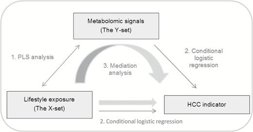
General scheme of the analytical framework developed in the study. A PC-PR2 analysis is carried out beforehand to identify relevant sources of variation. In the PLS model, the X- and Y-sets are related to each other, and scores are computed (1). X- and Y-scores are, in turn, associated to a case–control indicator of HCC status in conditional logistic regression models (2). A mediation analysis is carried out to explore the role of metabolomics in the association between lifestyle factors and risk of HCC (3).
Results
In the PC-PR2 analyses, a total of 17 and 14 principal components were retained to explain an amount of total variability exceeding 80% in metabolomics and lifestyle data, respectively. Figure 2 shows that the ensemble of explanatory variables accounted for 19.4 and 26.7% of total variance, respectively, in metabolomics and lifestyle data, of which the highest contributor was ‘country of origin’ with consistently 8 and 22%. PLS analysis was carried controlling for this variable.
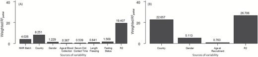
PC-PR2 analysis results* identifying the sources of variability in the NMR data (A) and in the lifestyle data (B).
* 17 and 14 components were retained to account for 80% (threshold used) of total NMR (A) and lifestyle variability (B), respectively. The R2 value represents the amount of variability in NMR/lifestyle variable explained by the ensemble of investigated predictors.
After a 7-fold cross-validation, three PLS factors were retained accounting for 21.7 and 8.5% of the overall variability observed in predictor and response variables, respectively (Table 1). Lifestyle variables and clusters of NMR variables contributing highly to PLS factors were identified using factor loading values (Table 2). The first PLS factor was predominantly positively associated with dairy products and cakes and biscuits intake, while lifetime alcohol intake, smoking status and diabetes displayed negative loadings for this lifestyle component (Table 2). On the same PLS factor, signals mainly associated with glucose and bonds of lipids with negative loading values, and with aspartate, glutamine and lysine with positive loadings emerged on the metabolomic profile (Table 2). Lifestyle variables characterising the second PLS factor included cereal products, height and education level with negative loadings, and hepatitis with positive loadings. The metabolic signature included NMR variables with positive loadings associated with aromatic amino acids (phenylalanine, tyrosine) and glucose; and those with negative loadings associated mainly with bonds of lipids, threonine and mannose (Table 2). The third PLS factor had a lifestyle pattern outlining intake of vegetables (high negative loadings values), lifetime alcohol consumption, smoking and hepatitis infection (positive loadings). Its counterpart NMR pattern highlighted signals of glucose and aspartate, with high negative loadings, along with signals of ethanol, myo-inositol, proline and glutamate as prominent metabolites with positive loadings (Table 2).
Individual and cumulative variation (%) explained by the first 3 PLS factors in 21 lifestyle (X-set) and 285 NMR (Y-set) variables
| # of PLS | Lifestyle variables | NMR variables | ||
|---|---|---|---|---|
| Factors | Individual | Cumulative | Individual | Cumulative |
| 1 | 6.17 | – | 5.51 | – |
| 2 | 6.23 | 12.40 | 2.38 | 7.89 |
| 3 | 9.27 | 21.67 | 0.59 | 8.48 |
| # of PLS | Lifestyle variables | NMR variables | ||
|---|---|---|---|---|
| Factors | Individual | Cumulative | Individual | Cumulative |
| 1 | 6.17 | – | 5.51 | – |
| 2 | 6.23 | 12.40 | 2.38 | 7.89 |
| 3 | 9.27 | 21.67 | 0.59 | 8.48 |
Lifestyle and NMR cluster variables contributing to each of the 3 PLS factors (N = 336, X-set = 21, Y-set = 285)
| PLS factor | Lifestyle variablea | Loading value | CS (ppm)a,b | Metabolitec | Loading value |
|---|---|---|---|---|---|
| 1 | Dairy products | 0.28 | 5.22 | Glucose | −0.06 |
| Cakes and biscuits | 0.32 | 3.88 | −0.05 | ||
| Lifetime alcohol consumption | −0.25 | 3.82 | −0.06 | ||
| Smoking status | −0.39 | 3.76 | −0.06 | ||
| Diabetes | −0.63 | 3.71 | −0.05 | ||
| 3.54 | −0.05 | ||||
| 3.50 | −0.07 | ||||
| 3.48 | −0.07 | ||||
| 3.44 | Acetoacetate | −0.07 | |||
| 3.23 | Choline + glycerphosphocholine | −0.04 | |||
| 3.01 | Lysine | 0.10 | |||
| 2.94 | Albumin | 0.10 | |||
| 2.65 | Aspartate | 0.10 | |||
| 2.42 | Glutamine | 0.10 | |||
| 2.28 | Acetoacetate | 0.10 | |||
| 2.22 | CH2–CH2–COOC bond of lipids + acetone | −0.04 | |||
| 1.86 | Lysine | 0.09 | |||
| 1.87 | 0.10 | ||||
| 1.53 | CH2–CH2–COOC bond of lipids | −0.03 | |||
| 2 | Cereal and cereal products | −0.16 | 7.17 | Tyrosine | 0.13 |
| Height | −0.34 | 6.87 | 0.13 | ||
| Education level | −0.26 | 5.27 | CH=CH bond of lipids | −0.13 | |
| Hepatitis | 0.49 | 5.22 | Glucose | 0.16 | |
| 5.18 | Mannose + lipid O–CH2 | −0.12 | |||
| 4.27 | Lipid O–CH2 | −0.12 | |||
| 4.25 | Threonine | −0.14 | |||
| 4.07 | Choline + lipid O–CH2 + myoinositol | −0.12 | |||
| 4.05 | Creatinine | −0.14 | |||
| 3.88 | Glucose | 0.15 | |||
| 3.82 | 0.16 | ||||
| 3.76 | 0.15 | ||||
| 3.71 | 0.15 | ||||
| 3.54 | 0.15 | ||||
| 3.50 | 0.16 | ||||
| 3.48 | 0.16 | ||||
| 3.44 | Acetoacetate | 0.16 | |||
| 3.23 | Choline + glycerophosphocholine | 0.15 | |||
| 2.80 | Aspartate | −0.12 | |||
| 2.22 | CH2–CH2–COOC bond of lipids + acetone | −0.11 | |||
| 2.19 | CH2–CH2–COOC bond of lipids | −0.15 | |||
| 2.02 | Proline + glutamate + CH2=C bonds of lipids | −0.13 | |||
| 1.53 | CH2–CH2–COOC bond of lipids | −0.13 | |||
| 1.25 | CH2 bond of lipids | −0.12 | |||
| 0.86 | Cholesterol + CH3 bond of lipids | −0.12 | |||
| 3 | Vegetables | −0.42 | 7.32 | Phenylalanine | 0.11 |
| Lifetime alcohol consumption | 0.29 | 5.22 | Glucose | −0.13 | |
| Smoking status | 0.25 | 4.28 | Lipid O–CH2 | 0.11 | |
| Hepatitis | 0.26 | 3.88 | Glucose | −0.11 | |
| 3.82 | −0.11 | ||||
| 3.76 | −0.12 | ||||
| 3.71 | −0.11 | ||||
| 3.69 | −0.11 | ||||
| 3.63 | Myoinositol | 0.16 | |||
| 3.50 | Glucose | −0.13 | |||
| 3.48 | −0.12 | ||||
| 3.44 | Acetoacetate | −0.12 | |||
| 3.35 | Proline | 0.11 | |||
| 3.33 | 0.13 | ||||
| 3.28 | Myoinositol | 0.12 | |||
| 3.23 | Choline + glycerophosphocholine | −0.12 | |||
| 2.80 | Aspartate | −0.13 | |||
| 2.76 | part of =CH–CH2–CH= bond of lipids | −0.13 | |||
| 2.35 | Proline + glutamate | 0.12 | |||
| 2.33 | 0.13 | ||||
| 1.20 | 3-hydroxybutyrate + CH2 bond of lipids | 0.11 | |||
| 1.16 | Ethanol | 0.15 | |||
| 0.66 | Cholesterol | 0.11 |
aRelevant lifestyle and NMR variables contributing to each PLS factor selected based on their associated loading values <10th percentile (pctl) and >90th pctl or <5th pctl and >95th pctl, respectively.
bCS: 1H chemical shift (ppm) of the cluster (centre value).
cSome of the identified clusters were found to be background noise during the annotation phase and were removed from this table.
Conditional logistic regression models relating HCC risk with the X- and Y-scores are shown in Table 3. The first PLS factor was associated to a non-significant decreased HCC risk (23 and 4% in the X- and Y-scores, respectively), while the second and third factors were associated to a statistically significant increased HCC risk (54 and 11%; and 37 and 22% respectively). Results for the ROC curves parameters are reported in Table 4, including AUC, sensitivity, specificity, accuracy and PPV for different combinations of the X- and Y-scores. The AUC of the X-scores and Y-scores for all 3 PLS factors, adjusted for C-reactive protein concentration, alpha-fetoprotein concentration and the score of liver damage, was 0.859 and 0.853, respectively. An increase in the resampled cross-validated AUC values was also observed for all three X- and Y-scores, albeit smaller, with 0.836 and 0.827, respectively. Results from the sensitivity analysis conducted on data excluding sets where cases were diagnosed within the first 2 years of follow-up, showed similarities in terms of lifestyle variables’ and metabolites’ loadings on the PLS factors (Supplementary Table 2, available at Mutagenesis Online). Notable differences pertained to the identification of new signals for the first PLS factor including ethanol, histidine and an unknown compound. On the second lifestyle factor, body mass index (BMI) (positive loadings) replaced education level (negative loadings) while the reflected metabolomic profile was comparable to its counterpart from the main analysis (Supplementary Table 2, available at Mutagenesis Online). On the third factor, smoking status and hepatitis (positive loadings) were replaced by sugar and confectionary intake (negative loadings); signals contributing to the associated metabolic profile remained the same but the direction of the association was inversed as loadings had opposite signs as compared to the counterpart PLS factor of the main model (Supplementary Table 2, available at Mutagenesis Online). Corresponding ORs from conditional logistic regression models relating the X- and Y-scores to HCC risk are available in Table 5. The scores showed a statistically significant association in the second factor for both sets and in the third factor for the Y-set. ROC-associated statistics for different models are presented in Supplementary Table 3, available at Mutagenesis Online. The VIP plot (Figure 3) displayed the results for the importance of the lifestyle variables in the prediction of the Y-set computed for the main PLS model performed including all subjects (A) and for the sensitivity model (B). The results suggested a potential gain in stability as prominent lifestyle variables for prediction were maintained (hepatitis/diabetes/cakes and biscuits), the magnitude of the VIP was improved for some (fat/lifetime alcohol intake) and less emphasis was put on others (BMI/physical activity).
HCC odds ratiosa and 95% confidence interval (OR, 95% CI) associated with the lifestyle (X-set) and the NMR clusters (Y-set) PLS scores in the main analysis (N = 336, X-set = 21, Y-set = 285)
| PLS lifestyle variables X-scores | PLS NMR Variables Y-scores | ||||
|---|---|---|---|---|---|
| Factor | ORb (95% CI) | P-Waldc | Factor | ORb (95% CI) | P-Waldc |
| 1 | 0.77 (0.58, 1.02) | 0.07 | 1 | 0.96 (0.91, 1.01) | 0.09 |
| 2 | 1.54 (1.06, 2.25) | 0.02 | 2 | 1.11 (1.02, 1.22) | 0.02 |
| 3 | 1.37 (1.05, 1.79) | 0.02 | 3 | 1.22 (1.04, 1.44) | 0.01 |
aModels were adjusted for C-reactive protein concentration, alpha-fetoprotein concentration and a composite score for liver damage. Cases and controls were matched on age at blood collection (± 1 year), sex, study centre, date (± 2 months) and time of the day at blood collection (± 3h), fasting status at blood collection (<3/3–6/>6h); among women, additional matching criteria included menopausal status (pre-/peri-/postmenopausal) and hormone replacement therapy use at time of blood collection (yes/no).
bORs expressing the change in HCC risk associated to 1SD increase in the score.
cWald’s test was for continuous exposure compared with a Chi-square distribution with 1 degree of freedom (dof).
Area under the curve (AUC), sensitivity, specificity, accuracy and positive predictive value (PPV) of ROC models (with 95% CI), from the main PLS analysis (N = 336, X-set = 21, Y-set = 285)
| AUC | AUCbb | Sensitivity | Specificity | Accuracy | PPV | |
|---|---|---|---|---|---|---|
| Adjustment covariates (ADJ)a | 0.842 (0.794, 0.891) | 0.821 (0.766, 0.868) | 0.752 (0.662, 0.829) | 0.802 (0.743, 0.852) | 0.785 | 0.0015 |
| X1 scores + ADJ | 0.846 (0.797, 0.894) | 0.825 (0.766, 0.875) | 0.743 (0.653, 0.821) | 0.838 (0.783, 0.884) | 0.806 | 0.0018 |
| X1 + X2 scores + ADJ | 0.854 (0.808, 0.900) | 0.831 (0.772, 0.881) | 0.743 (0.653, 0.821) | 0.824 (0.768, 0.872) | 0.797 | 0.0017 |
| X1 + X2 + X3 scores + ADJ | 0.859 (0.811, 0.907) | 0.836 (0.778, 0.887) | 0.796 (0.710, 0.866) | 0.788 (0.729, 0.840) | 0.791 | 0.0015 |
| Y1 scores + ADJ | 0.841 (0.793, 0.890) | 0.817 (0.760, 0.865) | 0.735 (0.643, 0.813) | 0.820 (0.763, 0.868) | 0.791 | 0.0016 |
| Y1 + Y2 scores + ADJ | 0.845 (0.795, 0.894) | 0.820 (0.762, 0.872) | 0.735 (0.643, 0.813) | 0.851 (0.798, 0.895) | 0.812 | 0.0020 |
| Y1 + Y2 + Y3 scores + ADJ | 0.853 (0.804, 0.902) | 0.827 (0.771, 0.877) | 0.726 (0.634, 0.805) | 0.883 (0.833, 0.922) | 0.890 | 0.0025 |
aThe model is run on the ADJ including the C-reactive protein concentration, alpha-fetoprotein concentration and a composite score for liver damage.
bAUCb is the bootstrapped-cross validated estimate of the AUC. X1, X2 and X3 are the lifestyle component scores of the first, second and third PLS factors, respectively. Y1, Y2, and Y3 are the metabolomics component of the first, second and third PLS factors, respectively.
HCC odds ratiosa and 95% confidence intervals (OR, 95%CI) associated with the lifestyle (X-set) and the NMR clusters (Y-set) PLS scores in the sensitivity analysis (N=271, 92 cases, 179 controls)
| PLS lifestyle variables X-scores | PLS NMR variables Y-scores | ||||
|---|---|---|---|---|---|
| Factor | ORb (95% CI) | P-Waldc | Factor | ORb (95% CI) | P-Waldc |
| 1 | 0.80 (0.60, 1.08) | 0.15 | 1 | 0.96 (0.94, 1.04) | 0.56 |
| 2 | 1.56 (1.02, 2.40) | 0.04 | 2 | 1.18 (1.03, 1.36) | 0.02 |
| 3 | 0.86 (0.67, 1.11) | 0.26 | 3 | 0.86 (0.73, 0.99) | <0.05 |
The sensitivity analysis was conducted excluding sets where cases were diagnosed within the first 2 years of follow-up (X-set = 21, Y-set = 285).
aModels were adjusted for C-reactive protein concentration, alpha-fetoprotein concentration and a composite score for liver damage. Cases and controls were matched on age at blood collection (± 1 year), sex, study centre, date (± 2 months) and time of the day at blood collection (± 3h), fasting status at blood collection (<3/3–6/>6h); among women, additional matching criteria included menopausal status (pre-/peri-/postmenopausal) and hormone replacement therapy use at time of blood collection (yes/no).
bORs expressing the change in HCC risk associated to 1SD increase in the score.
cWald’s test was for continuous exposure compared with a Chi-square distribution with 1 degree of freedom (dof).
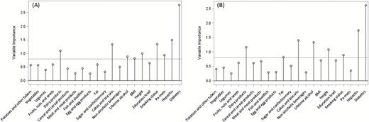
Variable importance plot (VIP) displaying the variable importance for projection statistic of the predictor variables for the PLS analyses. (A) Results from the main PLS model run on all observations (N = 336, X-set = 21, Y-set = 285). (B) Results from the PLS sensitivity analysis run on a subsample (N = 271, 92 cases, 179 controls) excluding sets where cases were diagnosed within the first 2 years of follow-up (X-set = 21, Y-set = 285). The horizontal line corresponds to Wold’s criterion (0.8), the threshold used to rule if a variable has an important contribution to the construction of the Y variables (see Supplementary Appendix, available at Mutagenesis Online for further details).
Finally, the NIE was assessed in the mediation analyses and the results are presented in Table 6. Overall, there was limited evidence that metabolomic signals mediated the association between lifestyle components and HCC risk in the first PLS factor. Evidence of a significant mediated effect by the Y-scores was found in the second and third PLS factors when models were adjusted for exposure–mediator interaction (Table 6).
Results from the mediation analysis (N = 336, X-set = 21, Y-set = 285): natural indirect effect (NIE) and 95%CIa
| Modelb | Natural indirect effect (NIE) | ||||
|---|---|---|---|---|---|
| Exposure (A) | Mediator (M) | Outcome | A*M interaction term | Estimate (95%CI) | P value |
| X1 score | Y1 score | HCC | No | 0.91 (0.77, 1.06) | 0.23 |
| X2 score | Y2 score | HCC | No | 1.11 (0.97, 1.25) | 0.12 |
| X3 score | Y3 score | HCC | No | 1.08 (0.94, 1.23) | 0.28 |
| X1 score | Y1 score | HCC | Yes | 0.96 (0.79, 1.17) | 0.70 |
| X2 score | Y2 score | HCC | Yes | 1.15 (1.01, 1.31) | 0.04 |
| X3 score | Y3 score | HCC | Yes | 1.13 (1.01, 1.28) | 0.04 |
aThe standard errors used to compute the 95% CI were obtained using the delta method.
bModels were adjusted for the C-reactive protein concentration, alpha-fetoprotein concentration and a composite score for liver damage, as well as for the other Y-scores, as potential mediator outcome confounders. Additionally, the outcome and the mediator models were adjusted for centre and age at blood collection.
Discussion
In this work, an analytical strategy based on PLS analysis was conceived to extract relevant information from sets of lifestyle and NMR metabolomic variables, and to relate the resulting components to the risk of disease. This offered a way to implement the MITM approach (6) in a nested case–control study on HCC within the EPIC study. MITM has been suggested as a way to link specific putative metabolites to lifestyle exposures and disease outcomes, thus leading to the identification of potential intermediate biomarkers (6).
An implementation of MITM was previously carried out in a nested case–control study in the Turin subcohort of EPIC (7) based on prospectively collected plasma samples from a pilot study on colon and breast cancers. In their work, a list of intermediate markers was identified by an in-parallel evaluation of the relationships between untargeted 1H NMR profiles with dietary exposures and risk of colon and breast cancers using correlation analysis and logistic regression. In our study, a different analytical framework was developed, largely exploiting features of PLS analysis, a multivariate technique that iteratively extracts components capturing covariability in sets of predictors and response variables (8,39). A set of lifestyle predictor variables were related to NMR responses. In a second step, PLS predictors’ and responses’ scores were linked to the risk of HCC.
Another sensitive issue in this analysis was the choice of lifestyle variables. Two disease-indicator variables reflecting environmental exposures, diabetes and hepatitis, were included in the set of predictors, as they turned out to have an important role in the characterisation of metabolomic signatures. In addition, diabetes is the main metabolic risk factor for HCC alongside with fatty liver disease (40,41), and chronic infection with hepatitis B (HBV) and particularly hepatitis C (HCV) viruses were classified as class I carcinogens for HCC by IARC (42).
Other relevant biomarkers were not part of the list of predictors in PLS analysis, but were controlled for in logistic regression models. This included C-reactive protein, alpha-fetoprotein and a score for liver damage, an index of different circulating enzymes measured in the hepatic tissue indicating potential underlying liver function impairment (25). The alpha-fetoprotein was included as an adjustment factor in the analyses not because of its established part as a serum marker for HCC diagnosis (26,43), but rather to account for it as a potential confounder that may cloud the relation between scores and HCC, both in conditional logistic regressions and in mediation analyses.
Similarly to other multivariate techniques, a key aspect of PLS analysis is the choice of the number of factors to retain, in an effort of exhaustively summarising data variability through a limited number of factors. Based on a 7-fold cross-validation, three linear combinations of variables were extracted in this work. A challenging aspect of this analysis is the interpretation of these factors, with respect to lifestyle and metabolomic variables. A subjective criterion based on the distribution of loading values was used throughout. The variables displaying the most extreme loading values (in absolute terms) were the ones characterising each factor.
The first lifestyle factor highlighted a healthy pattern with negative loadings for diabetes status, smoking status and lifetime alcohol intake, and was not associated to HCC risk, similarly to its metabolomics counterpart. The lifestyle component of the second PLS factor, was reflective of a lifestyle pattern reflective of ‘higher-risk exposures’, and was related to a significant 54% increase in HCC risk. Likewise, its associated metabolic component displayed a significant HCC risk augmentation by 11%. The lifestyle component of the third PLS factor described participants with lower vegetables intake, elevated lifetime alcohol consumption, more likely to be ever smokers and hepatitis positive; one standard deviation increase of this component was associated to a statistically significant 37% increase in HCC risk. Similarly, a 22% significant increase in HCC risk was observed for its metabolic counterpart, characterised by positive signals of ethanol and myoinositol, and displayed negative loadings for glucose.
The MITM is captured by the rationale of PLS analysis, in the sense that each set of lifestyle profiles and metabolic signatures of the extracted PLS factors mirrored one another. In addition, mediation was observed for the second and third PLS factors, whereby the metabolomic component mediated the relation between the lifestyle component and HCC, for which statistically significant associations with HCC risk were estimated, emphasising the presence of a MITM. Mediation analysis relies on the assumption that there is no mediator-outcome confounder that is affected by the exposure (34). In our study C-reactive protein, alpha-fetoprotein and liver damage score were weakly correlated to lifestyle factor score, thus introducing potential bias in the estimation of direct and indirect effects in our mediation analysis. Additionally, a number of background confounders (mediator-outcome and exposure-outcome confounders) were present that we have tried to control for, either by adjustments or by accounting for potential interactions, however some degree of bias can remain and caution should be employed when interpreting the results.
The predictive performance of PLS factors in relation to HCC occurrence was evaluated through an analysis of AUC values. The performance of the model improved progressively, with all 3 X- and Y-scores added; after a bootstrapped cross-validation, the AUC estimates were lower but the increase in the performance was nevertheless present. The ROC methodology allows estimation of PPV, which expresses the risk of disease after a positive test (44). In a setting with low HCC prevalence (π = 0.0004), in line with Western populations (45), extremely low PPV estimates were observed. In the absence of a very specific test, many false positive tests arise from disease-free individuals (44), thus leading to a dilution of PPV.
A sensitivity analysis was carried out excluding the first 2 years of follow-up, but results were virtually unchanged, both in terms of relative risk estimates in logistic regression models, and of percentage of variability explained in PLS analysis. These findings suggest that reverse causation bias, if present, was minimal.
This study had the ambition of integrating in the same analytical framework study participants’ lifestyle characteristics with a large number of NMR metabolic profiles. These data pose a number of methodological challenges due to their size and the complexity of exhaustively capturing and interpreting the biological processes they reflect. To address these issues, techniques involving multivariate statistics have been progressively revived in the recent years (2). Epidemiologic evaluations of metabolomic data frequently combined PLS with discriminant analysis, such as PLS-DA or O-PLS-DA. The main objective of these methods is to identify a series of metabolomic features distinguishing between two very distinct groups of study participants (46,47). In such strategies, only one set of variables is multidimensional and the response is one variable only. Similar multivariate techniques for pattern extraction, belonging to the family of regression methods, include reduced rank regression. This multivariate method relates an ensemble of response variables to a set of predictor variables where the estimated matrix of the regression coefficients is of reduced rank (48–50). In addition, canonical correlation analysis (CCA) (51) is a method applied to identify the optimum structure or dimensionality of each variable set that maximises the relationship between two sets of multi-dimensional variables. The main difference between CCA and PLS regression is that CCA maximises the correlation between the two new dimensions, i.e. extracted factors, whereas PLS maximises their covariance. PLS can be considered as a trade-off between CCA and PCA, since maximising the covariance corresponds to maximising the product of the correlation and standard deviation, given that cov(X,Y) = cor(X,Y)*SD(X)*SD(Y).
Untargeted NMR was used in this work to acquire metabolomic signals. Prior to PLS analysis, a bucketing procedure, the SRV (17,52), was applied to reduce the number of NMR variables to 285 clusters. This was done by aggregating consecutive NMR bins based on their covariance to correlation ratio. This allowed the identification of informative components of the spectra, thus acting as an efficient noise-removing filter. Subsequently the annotation effort remains challenging, for a number of reasons. The majority of published metabolomics studies often identified a limited number of metabolites at a time (53), and the Human Metabolome Database (HMDB) and other related resources (18,54), that offer richly annotated information continuously increasing the metabolite coverage for users, are mostly exploited through time consuming interactive procedures. In addition, individual metabolites often overlap in NMR signals, which can hinder annotations. These challenges, as well as large variability in metabolite concentrations, and disentangling informative signals from noise, are not specific to NMR and pertain to any type of untargeted technique. Such investigations may profit from complementary targeted metabolomic analytical strategies (54).
Throughout the different steps of this work, the scaling problem was first tackled by normalising spectra to total intensity. NMR data were also centred and Pareto-scaled, together with correction for potential batch effects (16). The PC-PR2 method offered a way to investigate major sources of systematic variability in NMR and lifestyle data (15). The variable ‘country of origin’ emerged as the variable accounting for the largest proportion of total variability, and the residual method was used to control for this variable in the following steps of the analysis. While this may lead to removing regional gradients of dietary variability, this step is instrumental to avoid unwanted systematic regional-specific bias in the data in country-specific questionnaire assessments. In addition, technical aspects like storage and handling of biological samples, fasting status at blood collection are specific to each country (15). In any case, variability due to ‘country of origin’ is not exploited in conditional logistic models, as cases and controls were also matched on centre.
One of the limitations of this study is the restricted sample size which raises concerns with regards to power to detect associations. While a larger sample size would possibly result in more statistically significant findings, we used the data that was available with NMR profiles measured. In this work, we have developed a framework to analyse complex data integrating lifestyle and metabolomics in relation to risk of disease. The approach described in this study has merits but also pitfalls among which it is worth mentioning that statistical methods are used repeatedly on the same set of data, notably the PLS model, the conditional logistic regression, the AUC estimation and mediation analysis. To partially address this, a cross-validation approach was devised for AUC estimation which involved conditional logistic regression, whereby PLS was done without knowledge of the case–control status. However, conditional logistic regression models and mediation analyses were implemented on the same data, and our analysis did not account for this limitation. This may have led to spuriously increase the nominal level of statistical significance of statistical tests.
Conclusion
The MITM emerged as a method for the identification of relevant biomarkers, with great potential to unravel utmost important steps in the aetiology of disease. The analytical strategy for MITM was developed to use all potentially informative aspects of high-throughput data by integrating metabolomic, dietary and lifestyle exposures together with disease indicators. While the framework was applied towards the investigation of HCC determinants, it can be easily extended to similar aetiological contexts and applied to other –omics settings.
Supplementary data
Supplementary Tables 1–3 and Appendix are available at Mutagenesis Online.
Funding
The coordination of EPIC is financially supported by the European Commission (DG-SANCO) and the International Agency for Research on Cancer. The national cohorts are supported by Danish Cancer Society (Denmark); Ligue Contre le Cancer, Institut Gustave Roussy, Mutuelle Générale de l’Education Nationale, Institut National de la Santé et de la Recherche Médicale (INSERM) (France); Deutsche Krebshilfe, Deutsches Krebsforschungszentrum and Federal Ministry of Education and Research (Germany); the Hellenic Health Foundation (Greece); Associazione Italiana per la Ricerca sul Cancro-AIRC-Italy and National Research Council (Italy); Dutch Ministry of Public Health, Welfare and Sports (VWS), Netherlands Cancer Registry (NKR), LK Research Funds, Dutch Prevention Funds, Dutch ZON (Zorg Onderzoek Nederland), World Cancer Research Fund (WCRF), Statistics Netherlands (The Netherlands); Nordic Centre of Excellence programme on Food, Nutrition and Health. (Norway); Health Research Fund (FIS), PI13/00061 to Granada), Regional Governments of Andalucía, Asturias, Basque Country, Murcia (no. 6236) and Navarra, ISCIII RETIC (RD06/0020) (Spain); Swedish Cancer Society, Swedish Scientific Council and County Councils of Skåne and Västerbotten (Sweden); Cancer Research UK (14136 to EPIC-Norfolk; C570/A16491 to EPIC-Oxford), Medical Research Council (1000143 to EPIC-Norfolk) (United Kingdom).
This work was supported by the French National Cancer Institute (L’Institut National du Cancer; INCA) [grant number 2009-139; PI: M. Jenab]. The work undertaken by N Assi was supported by the Université de Lyon I through a doctoral fellowship awarded by the EDISS doctoral school.
Acknowledgements
We would like to acknowledge the assistance of Dr Elodie Jobard from the ISA-CRMN in obtaining the annotation of the NMR data.
Conflict of interest statement: None declared.
References
